R语言代做编程辅导M3S2 Spring - Assessed Coursework:linear model(附答案)
原创R语言代做编程辅导M3S2 Spring - Assessed Coursework:linear model(附答案)
原创
全文链接:http://tecdat.cn/?p=30888
For this coursework you are required to download a dataset personal to you. Your dataset is available at: http://wwwf.imperial.ac.uk/~fdl06/M3S2_cw_2015/.RData where you must replace with your CID number. Any problems, email me. This dataset contains a dataframe called mydat | it consists of a response y and 3 columns of covariates x1, x2 and x3. Be aware!
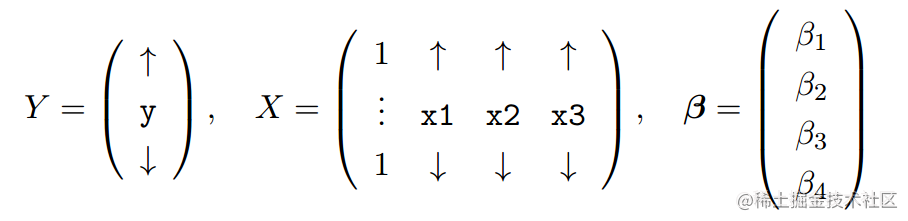
Q1) (a) In R fit the normal linear model with:
Based upon the summary of the model, do you think that the model fits the data well? Explain your reasoning using the values reported in the R summary | but do not include the whole summary in your report. (b) Perform a hypothesis test to ascertain whether or not to include the intercept term | use a 5% significance level. Include your code. (c) Conduct a hypothesis test comparing the models: E(Y ) = β1 against E(Y ) = β1 + β2x2 + β3x3 + β4x4 as a 5% level. Include your code. (d) By inspecting the leverages and residuals, identify any potential outliers. Name these data points by their index number. Give your reasoning as to why you believe these are potential outliers. You may present up to three plots if necessary
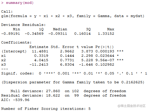
   mod=lm(y~x1+x2+x3,data=mydat)

summary(mod) 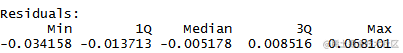
从残差值来看,拟合模型的预测值与实际数值差值较小,因此模型拟合较好。
常数项,x1,x2的p值均小于0.05,说明以上变量对y均有显著的影响。
从R-square值来看,该模型的拟合程度仍有提高的空间。B)#b.r
mod2=lm(y~x1+x2+x3-1,data=mydat)#删除常数项
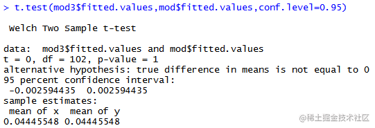
t.test(mod2$fitted.values,mod$fitted.values,conf.level=0.95)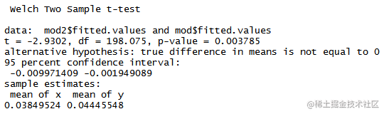
从检验结果来看,在5%的显著性水平上可以看到两个模型存在差异。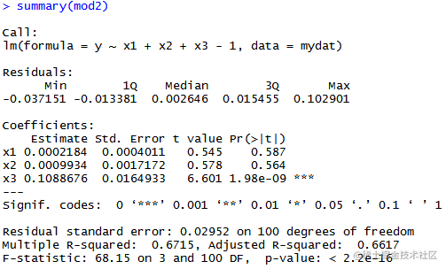
和模型1的拟合结果相比可以发现去除常数项后,模型2的R-squre要大于模型1,即拟合程度要好于模型1.C)#c.r
    mod3=lm(y~1)

summary(mod3)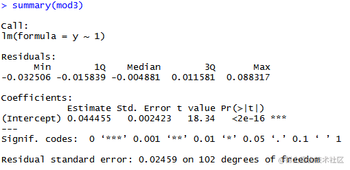
可以发现包含常数项和仅包含常数项的两个模型非常相似。P值大于0.05,因此可以接受原假设,即这两个模型是相似的。D)#d.r
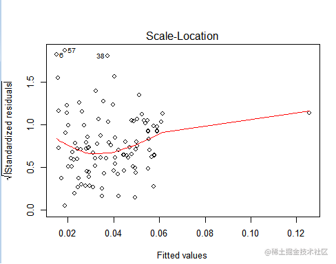
可以发现第6,57,38个样本的预测值与实际样本值的标准残差要大于其他值,因此可以认为6,57,38个样本为离群点。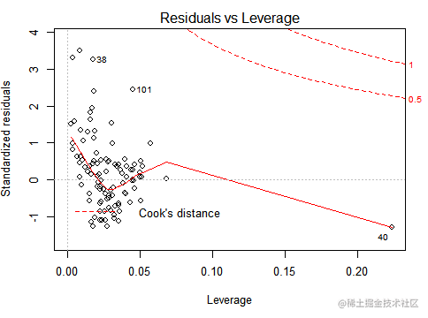
可以看到底38,101个样本对cook距离的值产生了较大的影响,明显不同与其他样本。因此

可以认为第38和101个样本对模型产生了影响,因此可以认为是离群点。
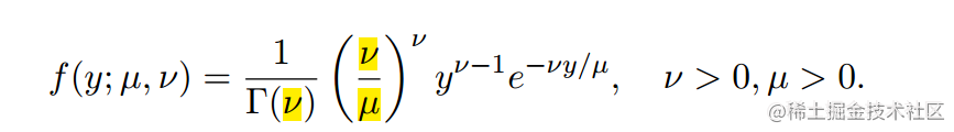
Q2) We shall now consider a GLM with a Gamma response distribution. (a) Show that a random variable Y where Y follows a Gamma distribution with probability density function:
(c) Rewrite (by \hand") the IWLS algorithm (similar to Algorithm 3.1 in notes on page 38) specifically for the Gamma response and using the link:

This is called the inverse link function. Continue to use the inverse link function for the remainder of the questions. (d) Write the components of the total score U1; : : : ; Up and the Fisher information matrix for this model. (e) Given the observations y, what is a sensible initial guess to begin the IWLS algorithm in general? (f) Manually write an IWLS algorithm to fit a Gamma GLM using your data, mydat, using the inverse link and same linear predictor in Q1a). Use the deviance as the convergence criteria and initial guess of β as (0:5; 0:5; 0:5; 0:5). Present your code and along with your final estimate of β and final deviance. (g) Based on your IWLS results, compute φbD and φbp and the estimates of var(βb2)
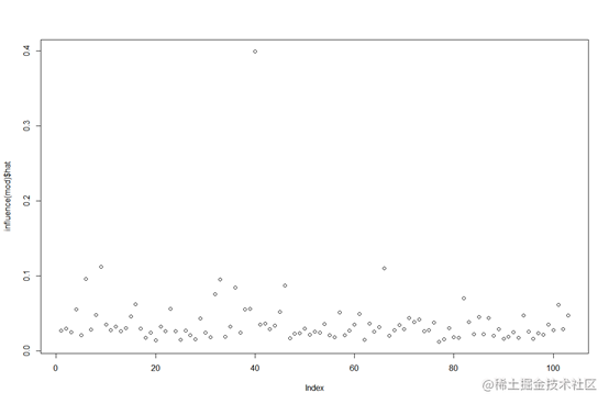
In R fit the model again with a Gamma response i.e. glm(y~x1+x2+x3,family=Gamma,data=mydat) Note the capital G in Gamma. Verify the results with your IWLS results. (h) Give a prediction for the response given by the model for x1= 13, x2= 5 x3= 0:255 and give a 91% confidence interval for this prediction. Include your code. (i) Perform a hypothesis test between this model and another model with the same link and response distribution but with linear predictor η where ηi = β1 + β2xi1 + β3xi2 for i = 1; : : : ; n: Use a 5% significance level. You may use the deviance function here. Include your code. (j) Using your IWLS results, manually compute the leverages of the observations for this model | present your code (but not the values) and plot the leverages against the observation index number. (k) Proceed to investigate diagnostic plots for your Gamma GLM. Identify any potential outliers | give your reasoning. Remove the most suspicious data point | you must remove 1 and only 1 | and refit the same model. Compare and comment on the change of the model with and without this data point | you may wish to refer to the relative change in the estimated coefficients. You may present up to three plots if necessary.
x3 <- mydat$x3
X=cbind(1,x1,x2,x3)
ilogit <- function(u)
? 1/(1+exp(-u))
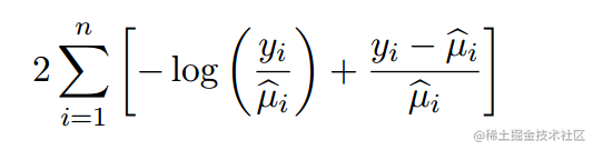
D <- function(mu){#deviance函数
? a <- (y-mu)/mu
? b <- -log(y/mu)
       G)#g.r

?

eta = cbind(1,x1,x2,x3)%*%beta

mu=1/(eta)

z = eta+((y-mu)/(-mu^2)) #form the adjusted variate

w = mu^2 #weights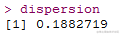
       H)#h.r

mod= glm(y~x1+x2+x3,family=Gamma,data=mydat)

?

? x1= 13 pp=predict(mod, newdata=data.frame(x1,x2,x3), level = 0.91, int = 'p')#用估计的参数对样本点进行预测
I)#i.r
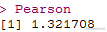
mod2=lm(y~x1+x2,data=mydat)
由于p值大于0.05,无法拒绝原假设H0,因此从deviance的差异度来看,可以认为两个模型并没有显著的差别。 J)#j.r
plot(mod)
       K)#k.r

y1=exp(beta[1]+beta[2]*x1+beta[3]*x2+beta[4]*x3)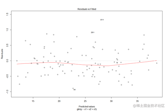
从残差拟合情况图来看,第44,28,81号样本点的残差值较大,可能为异常点,其中81号样本与拟合值的残差是最大的。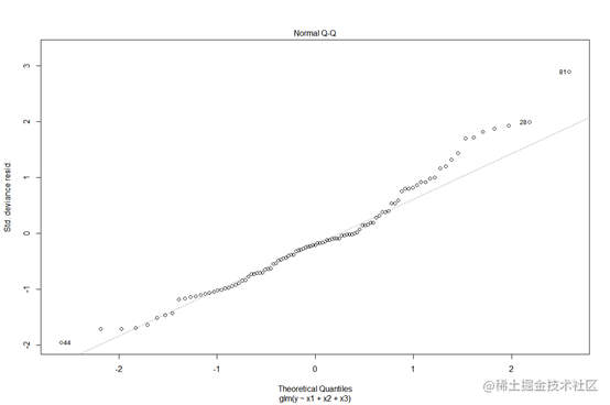
从正态分布qq图来看,大部分样本点分布在正态分布直线周围,可以认为样本点的总体服从正态分布。其中44,28,81号样本点里正态分布直线较远,因此可以认为其不符合正态分布,可能是离群点。从残差leverage图来看,第57,101,40号样本具有较大的cook距离,即都对我们的预测值产生了较大的影响。
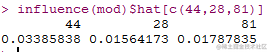
计算这3个样本的leverage统计量,可以发现第44号样本的值大于其他连个样本,因此认为第44号样本为异常点,可以删去。对比删去44号样本的模型和原来的模型
       mod2=lm(y~x1+x2+x3, family = Gamma,data=mydat1)

summary(mod2)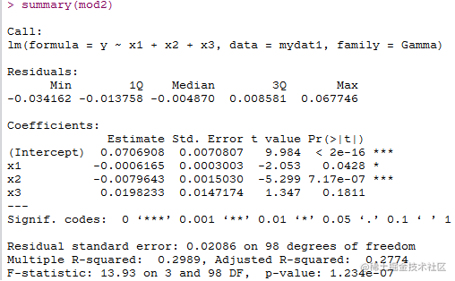
可以看到修改后的模型deviance residuals值减少了,不同变量对因变量的影响也更加显著,因此模型的拟合度提高。
原创声明:本文系作者授权腾讯云开发者社区发表,未经许可,不得转载。
如有侵权,请联系 cloudcommunity@tencent.com 删除。
原创声明:本文系作者授权腾讯云开发者社区发表,未经许可,不得转载。
如有侵权,请联系 cloudcommunity@tencent.com 删除。