单细胞空间联合分析之SpatialScope
原创单细胞空间联合分析之SpatialScope
原创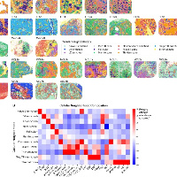
追风少年i
发布于 2024-04-15 11:48:38
发布于 2024-04-15 11:48:38
作者,Evil Genius
今天有人问我,HD的出现是否会取代visium,我个人觉得短期不会,visium和HD会并行存在很长时间,现有的visium数据也也很大部分没有分析完。
空间邻域的分析被这群大佬们玩出花来了,原始只是配受体、细胞类型,现在把转录因子、细胞通路、微生物、代谢数据全部放进来研究邻域了,牛的。

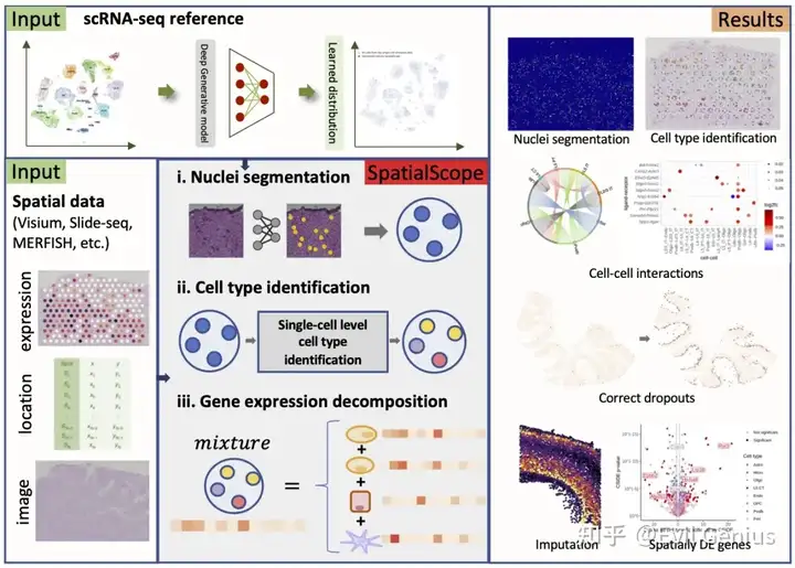
今天周一,不想干活,就看看这个有一些特点的单细胞空间分析软件SpatialScope吧,这个软件的分析结果跟之前的有一点点不一样。
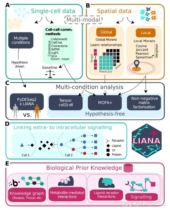
文章在Integrating spatial and single-cell transcriptomics data using deep generative models with SpatialScope(NC,IF 16.6)
看一眼教程
import numpy as np
import pandas as pd
import pathlib
import matplotlib.pyplot as plt
import matplotlib as mpl
import seaborn as sns
import scanpy as sc

import sys
sys.path.append('../src')
from utils import *

import warnings
warnings.filterwarnings('ignore')
Preprocessing scRNA-ref
ad_sc = sc.read('global_raw.h5ad')

ad_sc = ad_sc[ad_sc.obs['cell_type']!='doublets']
ad_sc = ad_sc[ad_sc.obs['cell_type']!='NotAssigned']
ad_sc = ad_sc[ad_sc.obs['cell_type']!='Mesothelial']
ad_sc = ad_sc[ad_sc.obs['cell_source']=='Sanger-Nuclei']

cell_type_column = 'cell_type'

sc.pp.filter_cells(ad_sc, min_counts=500)
sc.pp.filter_cells(ad_sc, max_counts=20000)
sc.pp.filter_genes(ad_sc, min_cells=5)
ad_sc = ad_sc[:,~np.array([_.startswith('MT-') for _ in ad_sc.var.index])]
ad_sc = ad_sc[:,~np.array([_.startswith('mt-') for _ in ad_sc.var.index])]

ad_sc = ad_sc[ad_sc.obs['donor']=='D2'].copy() # reduce batch effect among doners
ad_sc = ad_sc[ad_sc.obs.index.isin(ad_sc.obs.groupby('cell_type').apply(
    lambda x: x.sample(frac=3000/x.shape[0],replace=False) if x.shape[0]>3000 else x).reset_index(level=0,drop=True).index)].copy()

ad_sc.X.max(),ad_sc.shape

sns.set_context('paper',font_scale=1.6)
fig, axs = plt.subplots(1, 1, figsize=(10, 10))
sc.pl.umap(
    ad_sc, color=cell_type_column, size=15, frameon=False, show=False, ax=axs,legend_loc='on data'
)
plt.tight_layout()
ad_sc.raw = ad_sc.copy()
sc.pp.normalize_total(ad_sc,target_sum=2000)

sc.pp.highly_variable_genes(ad_sc, flavor='seurat_v3',n_top_genes=1000)
sc.tl.rank_genes_groups(ad_sc, groupby=cell_type_column, method='wilcoxon')
markers_df = pd.DataFrame(ad_sc.uns["rank_genes_groups"]["names"]).iloc[0:100, :]
markers = list(np.unique(markers_df.melt().value.values))
markers = list(set(ad_sc.var.loc[ad_sc.var['highly_variable']==1].index)|set(markers)) # highly variable genes + cell type marker genes

ligand_recept = list(set(pd.read_csv('../extdata/ligand_receptors.txt',sep='\t').melt()['value'].values))
# if scRNA-seq reference is from human tissue, run following code to make gene name consistent
ligand_recept = [_.upper() for _ in ligand_recept]
add_genes = 'DCN GSN PDGFRA\
RGS5 ABCC9 KCNJ8\
MYH11 TAGLN ACTA2\
GPAM FASN LEP\
MSLN WT1 BNC1\
VWF PECAM1 CDH5\
CD14 C1QA CD68\
CD8A IL7R CD40LG\
NPPA MYL7 MYL4\
MYH7 MYL2 FHL2\
DLC1 EBF1 SOX5\
FHL1 CNN1 MYH9\
CRYAB NDUFA4 COX7C\
PCDH7 FHL2 MYH7\
PRELID2 GRXCR2 AC107068.2\
MYH6 NPPA MYL4\
CNN1 MYH9 DUSP27\
CKM COX41L NDUFA4\
DLC1 PLA2GS MAML2\
HAMP SLIT3 ALDH1A2\
POSTN TNC FAP\
SCN7A BMPER ACSM1\
FBLN2 PCOLCE2 LINC01133\
CD36 EGFLAM FTL1\
CFH ID4 KCNT2\
PTX3 OSMR IL6ST\
DCN PTX3 C1QA\
NOTCH1 NOTCH2 NOTCH3 NOTCH4 DLL1 DLL4 JAG1 JAG2\
CDH5 SEMA3G ACKR1 MYH11'.split()+['TNNT2','PLN','MYH7','MYL2','IRX3','IRX5','MASP1'] # some important genes that we interested

markers = markers+add_genes+ligand_recept
ad_sc.var.loc[ad_sc.var.index.isin(markers),'Marker'] = True
ad_sc.var['Marker'] = ad_sc.var['Marker'].fillna(False)
ad_sc.var['highly_variable'] = ad_sc.var['Marker']

sc.pp.log1p(ad_sc)
sc.pp.pca(ad_sc,svd_solver='arpack', n_comps=30, use_highly_variable=True)

sc.pp.neighbors(ad_sc, metric='cosine', n_neighbors=30, n_pcs = 30)
sc.tl.umap(ad_sc, min_dist = 0.5, spread = 1, maxiter=60)
fig, axs = plt.subplots(1, 1, figsize=(10, 10))
sc.pl.umap(
    ad_sc, color=cell_type_column, size=15, frameon=False, show=False, ax=axs,legend_loc='on data'
)
plt.tight_layout()
fig, axs = plt.subplots(1, 1, figsize=(10, 10))
sc.pl.umap(
    ad_sc, color="cell_states", size=10, frameon=False, show=False, ax=axs,legend_loc='on data'
)
plt.tight_layout()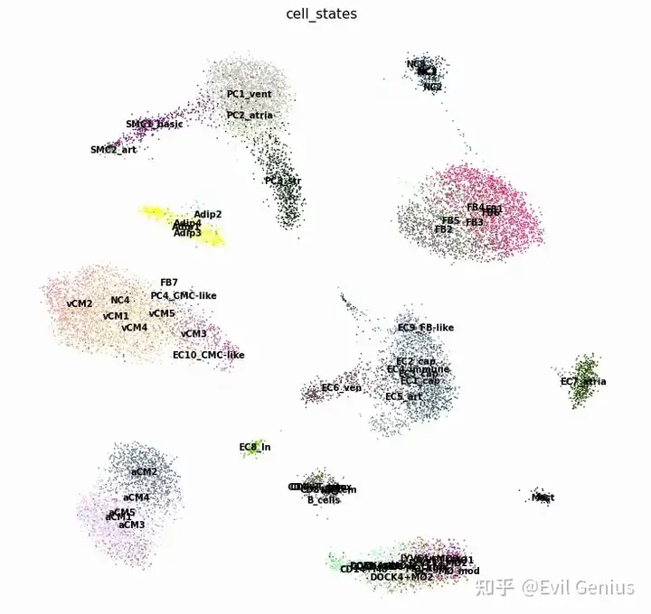
Learning the gene expression distribution of scRNA-seq reference using score-based model
python ./src/Train_scRef.py \
--ckpt_path ./Ckpts_scRefs/Heart_D2 \
--scRef ./Ckpts_scRefs/Heart_D2/Ref_Heart_sanger_D2.h5ad \
--cell_class_column cell_type \
--gpus 0,1,2,3 \
--sigma_begin 50 --sigma_end 0.002 --step_lr 3e-7
Run SpatialScope
Step1: Nuclei segmentation,10X的数据
python ./src/Nuclei_Segmentation.py --tissue heart --out_dir ./output --ST_Data ./demo_data/V1_Human_Heart_spatial.h5ad --Img_Data ./demo_data/V1_Human_Heart_image.tifStep2: Cell type identification
python ./src/Cell_Type_Identification.py --tissue heart --out_dir ./output --ST_Data ./output/heart/sp_adata_ns.h5ad --SC_Data ./Ckpts_scRefs/Heart_D2/Ref_Heart_sanger_D2.h5ad --cell_class_column cell_typeStep3: Gene expression decomposition
python ./src/Decomposition.py --tissue heart --out_dir ./output --SC_Data ./Ckpts_scRefs/Heart_D2/Ref_Heart_sanger_D2.h5ad --cell_class_column cell_type --ckpt_path ./Ckpts_scRefs/Heart_D2/model_5000.pt --spot_range 0,1000 --gpu 0,1,2,3
python ./src/Decomposition.py --tissue heart --out_dir ./output --SC_Data ./Ckpts_scRefs/Heart_D2/Ref_Heart_sanger_D2.h5ad --cell_class_column cell_type --ckpt_path ./Ckpts_scRefs/Heart_D2/model_5000.pt --spot_range 1000,2000 --gpu 0,1,2,3
python ./src/Decomposition.py --tissue heart --out_dir ./output --SC_Data ./Ckpts_scRefs/Heart_D2/Ref_Heart_sanger_D2.h5ad --cell_class_column cell_type --ckpt_path ./Ckpts_scRefs/Heart_D2/model_5000.pt --spot_range 2000,3000 --gpu 0,1,2,3
python ./src/Decomposition.py --tissue heart --out_dir ./output --SC_Data ./Ckpts_scRefs/Heart_D2/Ref_Heart_sanger_D2.h5ad --cell_class_column cell_type --ckpt_path ./Ckpts_scRefs/Heart_D2/model_5000.pt --spot_range 3000,4000 --gpu 0,1,2,3
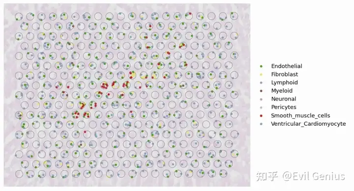
python ./src/Decomposition.py --tissue heart --out_dir ./output --SC_Data ./Ckpts_scRefs/Heart_D2/Ref_Heart_sanger_D2.h5ad --cell_class_column cell_type --ckpt_path ./Ckpts_scRefs/Heart_D2/model_5000.pt --spot_range 4000,4220 --gpu 0,1,2,3Cell type identification result at single-cell resolution for the whole slice
ad_sc = sc.read('../Ckpts_scRefs/Heart_D2/Ref_Heart_sanger_D2.h5ad')
ad_sp = sc.read('../output/heart/sp_adata.h5ad')

ad_sp.uns['cell_locations'].head()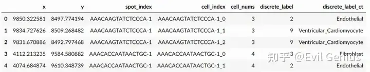
color_dict = {'Adipocytes': '#1f77b4',
 'Atrial_Cardiomyocyte': '#ff7f0e',
 'Endothelial': '#2ca02c',
 'Fibroblast': '#F5DE7E',
 'Lymphoid': '#9D9BC2',
 'Myeloid': '#8c564b',
 'Neuronal': '#D29D9E',
 'Pericytes': '#BDBDBD',
 'Smooth_muscle_cells': '#d62728',
 'Ventricular_Cardiomyocyte': '#7AA4C1'}
fig, ax = plt.subplots(1,1,figsize=(12, 8),dpi=100)
PlotVisiumCells(ad_sp,"discrete_label_ct",size=0.7,alpha_img=0.2,lw=0.3,palette=color_dict,ax=ax)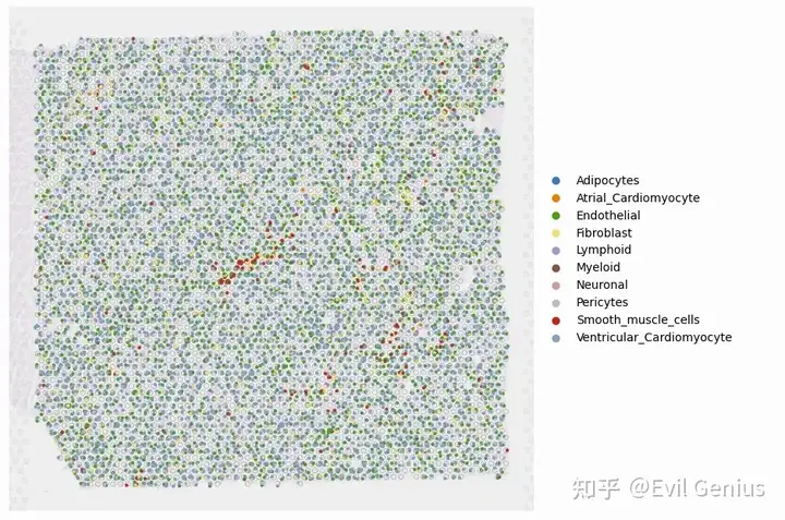
Inferred cell type compositions
p2_res = ad_sp.uns['cell_locations']
ss = pd.DataFrame(p2_res.discrete_label_ct.value_counts()/p2_res.shape[0])
ss.columns = ['SpatialScope']


alignres_cytospace = pd.read_csv('/home/share/xiaojs/spatial/sour_sep/heart/res/cytospace/D2/cytospace_results/assigned_locations.csv')
cs = pd.DataFrame(alignres_cytospace['CellType'].value_counts()/alignres_cytospace.shape[0])
cs.columns = ['CytoSpace']

tg = pd.read_csv('/home/share/xiaojs/spatial/sour_sep/heart/res/Tangram_P2_D2Ref_nu10.csv',index_col=0)
tg = pd.DataFrame(tg['cluster'].value_counts()/tg.shape[0])
tg.columns = ['Tangram']

df_res = ss.merge(tg,left_index=True,right_index=True,how='outer').merge(cs,left_index=True,right_index=True,how='outer')
df_res = df_res.fillna(0).T
df_res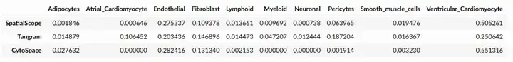
# variables
plot_columns = ['Ventricular_Cardiomyocyte','Atrial_Cardiomyocyte',
 'Endothelial',
 'Fibroblast',
 'Pericytes',
 'Smooth_muscle_cells',
 'Myeloid',
 'Lymphoid',
 'Neuronal',
 'Adipocytes']
plot_colors = [color_dict[_] for _ in plot_columns]

labels = plot_columns#df_res.columns
colors = plot_colors#['#1D2F6F', '#8390FA', '#6EAF46', '#FAC748']
title = 'Video Game Sales By Platform and Region\n'
subtitle = 'Proportion of Games Sold by Region'
def plot_stackedbar_p(df, labels, colors, title, subtitle):
    fields = labels#df.columns.tolist()

    # figure and axis
    sns.set_context('paper',font_scale=1.8)
    fig, ax = plt.subplots(1, figsize=(18, 4),dpi=100)
# plot bars
    left = len(df) * [0]
    for idx, name in enumerate(fields):
        plt.barh(df.index, df[name], left = left, color=colors[idx])
        left = left + df[name]
# legend
    plt.legend(labels, bbox_to_anchor=([.95, -0.14, 0, 0]), ncol=5, frameon=False)
# remove spines
    ax.spines['right'].set_visible(False)
    ax.spines['left'].set_visible(False)
    ax.spines['top'].set_visible(False)
    ax.spines['bottom'].set_visible(False)
# format x ticks
    xticks = np.arange(0,1.1,0.1)
    xlabels = ['{}%'.format(i) for i in np.arange(0,101,10)]
    plt.xticks(xticks, xlabels)
# adjust limits and draw grid lines
    plt.ylim(-0.5, ax.get_yticks()[-1] + 0.5)
    ax.xaxis.grid(color='gray', linestyle='dashed')
plt.show()

plot_stackedbar_p(df_res, labels, colors, title, subtitle)
import squidpy as sq
image = plt.imread('../demo_data/V1_Human_Heart_image.tif')

img = sq.im.ImageContainer(image)
crop = img.crop_corner(0, 0)

inset_x = int(img.shape[0]*(4.1/10)) # column
inset_y = int(img.shape[1]*(4.6/10)) # row
inset_sx = int(img.shape[0]*(2/10))
inset_sy = int(img.shape[1]*(1.6/10))

ad_sp_crop = ad_sp[
    (ad_sp.obsm["spatial"][:, 0] > inset_x) & (ad_sp.obsm["spatial"][:, 1] > inset_y)
    & (ad_sp.obsm["spatial"][:, 0] < inset_x+inset_sx) & (ad_sp.obsm["spatial"][:, 1] < inset_y+inset_sy), :
].copy()

ad_sp_crop.uns['cell_locations'] = ad_sp_crop.uns['cell_locations'].loc[ad_sp_crop.uns['cell_locations'].spot_index.isin(ad_sp_crop.obs.index)].reset_index(drop=True)
fig, ax = plt.subplots(1,1,figsize=(12, 8),dpi=100)
PlotVisiumCells(ad_sp_crop,"discrete_label_ct",size=0.3,alpha_img=0.3,lw=0.8,palette=color_dict,ax=ax)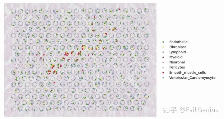
后续还有marker gene的展示,大家自己看吧。

示例在SpatialScope,https://spatialscope-tutorial.readthedocs.io/en/latest/index.html.
生活很好,有你更好
原创声明:本文系作者授权腾讯云开发者社区发表,未经许可,不得转载。
如有侵权,请联系 cloudcommunity@tencent.com 删除。
原创声明:本文系作者授权腾讯云开发者社区发表,未经许可,不得转载。
如有侵权,请联系 cloudcommunity@tencent.com 删除。
评论
登录后参与评论
推荐阅读
目录